Training the YOLOv5 Object Detector on a Custom Dataset

YOLO stands for You Only Look Once. Before the inception of YOLO, object detection repurposed classifiers to perform detection. YOLO, however, frames object detection as a regression problem to spatially separated bounding boxes and any associated class probabilities. A single neural network predicts the probabilities for all the predicted bounding boxes. There is different versions of the network, processing an astounding 155 frames per second. It has been proved to outperform other methods including DPM, R-CNN, when generalizing from natural images to other domains like artwork. YOLOv5 version in the YOLO family is written ground up in PyTorch. It is also ~90 percent smaller than YOLOv4.

Object detection progression

The current domain specific object detectors can usually be divided into two categories. One of the prominent two-stage detectors is Faster R-CNN. It builds on a first stage called RPN, meaning Regional Proposal Network to predict any bounding boxes. The second stage is Rol pooling operation from each predicted bounding box for the classification and regression tasks. On the contrary, there is one-stage detectors like YOLO and SSD. Two-stage detectors provide high localization and object recognition accuracy, whereas one-stage detectors provide higher speeds with lower interference. A one-stage detector like YOLO propose predicted bounding boxes from the input image directly without regional proposal step (RPN), thus making them time efficient and can be used real-time with minimal lag time.

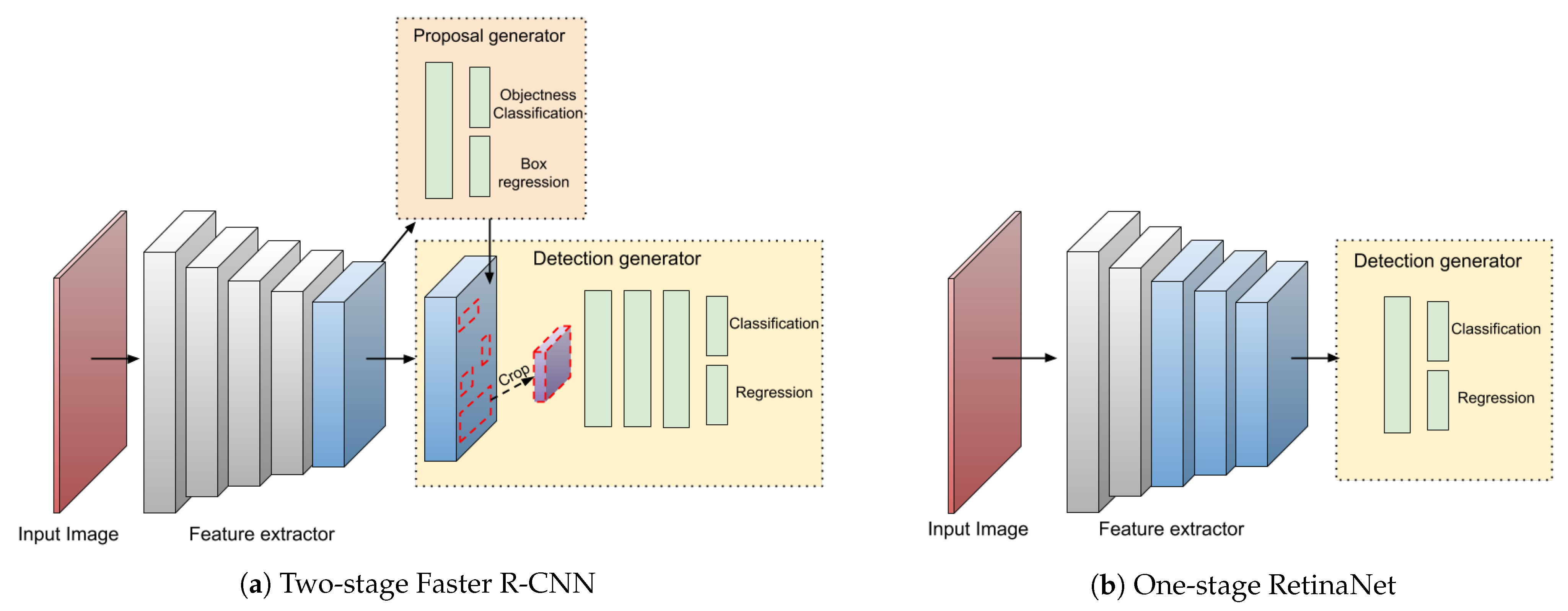
Figure 1

Figure 1 (a) depicts the basic architecture of a two-stage detector which consists of a RPN to feed region proposals into classifiers and regressor. Figure (b) however, predicts bounding boxes directly from input images. The light grey boxes are a multitude of convolutional layers with the same resolution of a backbone network, as it gets down sampled after each operation.

YOLOv5 architecture

YOLO processes an image using a single neural network, and then separates it into parts and predicts bounding boxes and probabilities for each component. These boxes have weights for anticipated probabilities. The predictions are only made through a single forward propogation into the neural network. The detected items are delivered after a non-max supression ensuring that the algorithm only detects an object once.

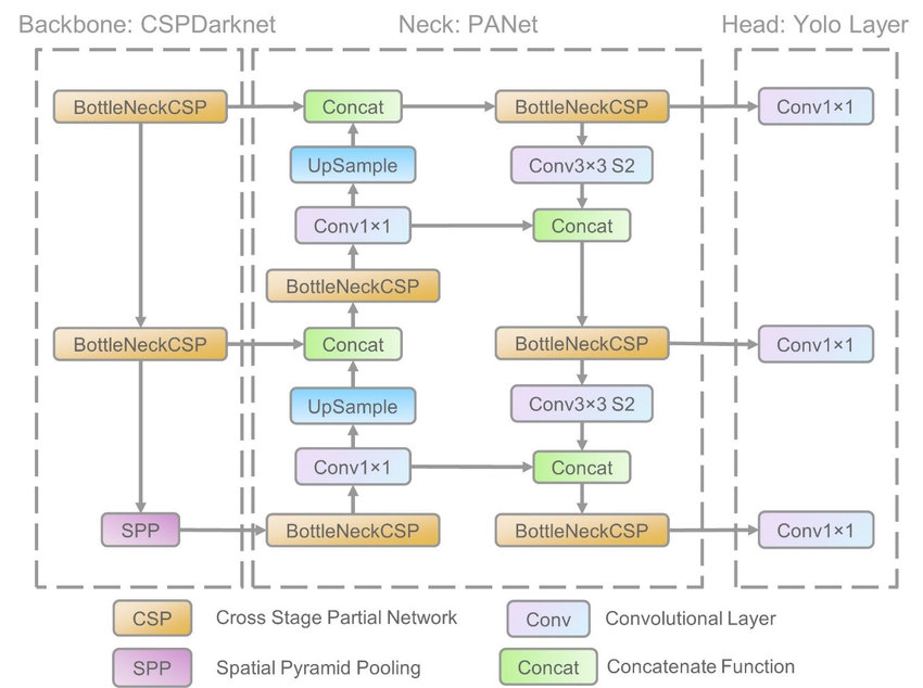
Figure 2 (src)

The model consists of three main blocks as shown in Figure 2 above.

1. Backbone: It employs CSPDarknet to extract features from the images of cross-stage partial networks.

2. Neck: PANet is used to generate a feature pyramid network to perform regression analysis on the features and pass it to the next block.

3. Head: This YOLO convulational layer makes predictions from the anchor boxes for object detection and assigns weights.

YOLOv5 pre-trained models

There are several pretrained models to select from. There is a trade-off between the size of the model and time interference. The YOLOv5s is just 14MB but is not as accurate. But the YOLOv5x is most accurate with a size of 166MB. What model to pick for your project solely depends on the scope and production requirements.

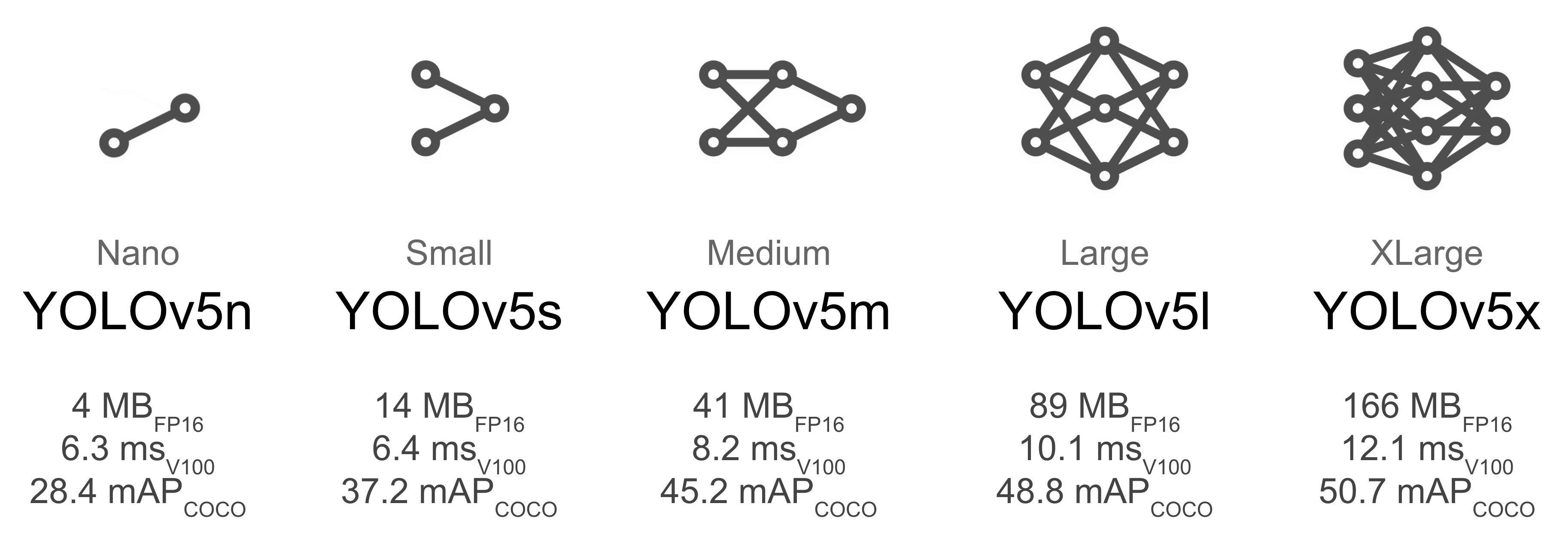
Figure 3 (src)

We can see the COCO mean average precision value increase as you pick the heavier models for training.

Training A Custom Dataset (project)

Setting up YOLOv5

Let us set up YOLO on the local machine. The following guide will get you started either on Windows 10/11 or Ubuntu 18.04. If you rather prefer a virtual environment, below is also a link to Google CoLab notebook.

If not already, install Python from this link for your OS to move ahead in this tutorial.

Install some dependencies using pip. Install Tensorflow, Tensorboard, and Torch by running the follow commands in the console.

    python -m pip install --upgrade pip
    pip install tensorflow==2.3.1 
    pip install tensorboard==2.4.1
    pip install torch
    

Prepping a custom dataset

The models must be trained on labelled data in order to learn classes of objects in that data. You could either manually prepare your dataset or get a pre-labelled data online.

1. Use Roboflowto label, prepare, or get a custom data in YOLO compatible format.

2. I personally like to use LabelImg as it is open-source and just gets the job done. You can easily load the directory where your pictures live, and keep annotating using the GUI.

Training the dataset

1. Create a folder on your Desktop to house the YOLOv5 repository.

2. Clone the repository from Ultralytics by running the command:

   
       git clone https://github.com/ultralytics/yolov5
       

   cd into the yolov5 folder on your terminal.

3. Install all the dependencies from the `requirements.txt` file by running the below command:

       
       pip install -r requirements.txt
       
       

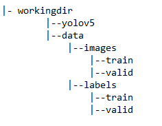
The tree structure above is how I like to set my pictures up before starting the training. Within the cloned yolov5 repo, I create a folder called `data`. This will house all the image files (any supported extentions), and the .txt files that hold the bounding box coordinates. The `image` folder inside `data`, has two sub-directories `train` and `val`. The `train` folder houses the training images, and `val` folder the validation images we provide to the model to generate the Precision, Recall, and mAP number by comnparing with the user specified ideal outcomes. The corresponding bounding boxes (.txt files) live in the `labels` folder in the same format.

Next, we create `data.yaml` in the yolov5 directory that instructs the model about our dataset. Here is a sample file:

    
    #yolov5/data.yaml

    train: data/images/train
    val: data/images/val

    # number of classes
    nc: 1

    # class names
    names: ['Pole']
    
    

You can have multiple classes depending on what you are trying to identfy in the dataset. In your labelled dataset, for example, you annoted classes for a face-mask, and no-face-mask. Then nc would have a value of 2, and the names array would have the name of the class.

Next, we train the network. We use various flags to set options regarding training:

1. img: This is size of the image. The original image will be resized while maintaining the aspect ratio

2. batch: The batch size

3. epochs: The number of epochs to train for (more info on epoch is available online)

4. data: A reference to the `data.yaml` that we just created

5. workers: Number of CPU workers

6. weights: Pretrained weights you want to start the training from. If training from scratch, use --weights `location of the file`

    
    python train.py --img 415 --batch 16 --epochs 30 --data data.yaml --weights models/yolov5s.pt --cache
    
    

This command will first cache the images and labels, and start running for the number of epochs specified. It creates a `runs` folder in the root that has all the logs and training results, including weight files. We use the weights file to detect later down the road using the model.

Monitoring ML workflow

We can also leverage Tensorbord that we installed in the beginning. This tool provides the measurments and visualizations needed during the machine learning workflow. You can monitor in real time the Precision, Recall, and mAP numbers as the epochs progress. Do make sure to run this as the epochs are in progress. Run the following command:

    
    load_ext tensorboard
    tensorboard --logdir runs
    
    

Tensorboard will run locally on port 6006 as a dashboard.

Detect using the model

There are multiple ways to run interference using the `detect.py` file. The --source flag defines the source of our detector, which can be a single image, a folder full of images, a video or a webcam.

To run interference over our dataset:

    
    python detect.py --source testPic.jpg --weights runs/train/exp/best.pt
    
    

Project reference